Worldlines - An Interactive Special Relativity Visualization

The goal of the axes scene (Figure 1) is to show how the system of rest coordinates for a moving particle are mapped into the rest frame of other particles - here, the “world frame” - within which the first particle is moving. The basis vectors for the world frame are labeled

(x, y, c t)

; and those for the moving particle are labeled

(x', y', c t')

The vector

c t'

represents the particle's 3-velocity - here through the (2+1) Minkowski space, analogous to the 4-velocity in real-world 4D spacetime. The point is that

c t'

is always tangent to the particle's path, and shows where the particle will be if it keeps its current velocity. The vector

c t'

is notable because in SR, it is not generally perpendicular to the

x' y'

plane in all frames of reference. That is, space and time between different frames are mixed - motion only along time (parallel to

c t'

) for the moving particle in frame

S'

has a changing spatial component in frame

S

(along

x

in Figure 1).

For any frame

S'

, the

x' y'

plane gives the surface of simultaneity; events in this plane are simultaneous for observers within the frame. The phenomena of relativity of simultaneity refers to the fact that given events A, B, and C such that A and B are simultaneous in frame

S

, and B and C are simultaneous frame

S'

, events A and C will generally not be simultaneous in either frame

S

S'

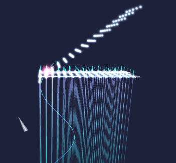
The axes scene (Figure 2) begins with a few simple particles at rest for reference, and a single “driven particle” whose velocity component

v_{x}

is defined as a sine wave oscillating between

0

and

0.99 c

, completing a cycle every

200 s

in the world frame. The driven particle has been made the “target particle”, meaning it's tracked by the camera, and that any coordinate (Lorentz) transforms later activated for display will be done for

γ

between it and the world frame.

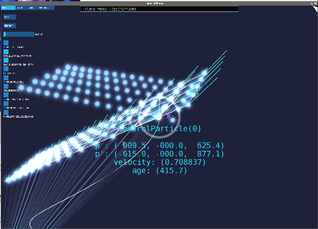
Clicking on the particle selects it, showing its identification and some information about its state. In Figure 3 for example, we see an already dramatically stretched axes at

0.95 c

nearly completely collapses with just a

~ 0.037 c

increase to

0.988 c

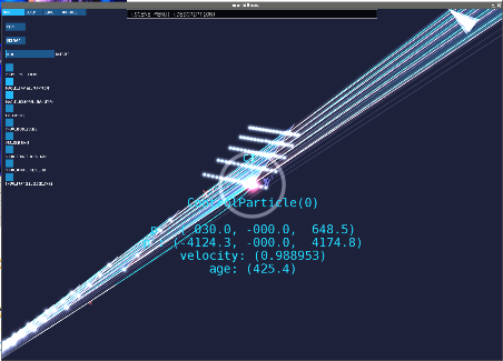
In Figure 4, the particle is again at

0.95 c

, but now the Lorentz transforms have been activated - meaning the coordinate space used for display now matches the space of the target particle. This is why the

c t'

and

x'

basis vectors again appear orthogonal (even at this high speed), since we are now in the the rest frame of the particle. The

c t

and

x

basis have been skewed in the opposite directions, stretching off-screen.

Figure 3:

In the world frame, the

x' c t'

axes grid of target particle collapses as the particle approaches

c

. Here the velocity increases from

0.9509

0.9878 c

Figure 4:

In the rest frame of the target particle, the target's coordinate space (and

x' c t'

axes grid) is undisturbed, even at high velocities, while the

x c t

basis (positioned at the target's location) skew away from the

x' c t'

grid, stretching offscreen.

2.2 Twin Paradox Scene

Figure 5:

The Twin Paradox Scene in the world frame, return stage. Twin A stays at rest, while twin B departs and returns at constant velocity. The conundrum goes as follows. If, as according to time dilation, “frames in relative motion see each other's clocks as advancing more slowly,” then what is the relationship between the ages of the two twins in this scenario?

Figure 6:

Twin Paradox Scene, departure stage. In twin A's frame, twin B is always aging more slowly. The yellow “ageDiff” meter tracks their difference in age,

Δ τ_{A - B}

, for the current simulation step as seen in the world frame. (Red clock ticks are spaced at

1 s

intervals; yellow ticks at

10 s

intervals. See Section 3.2.3 Graphical Elements: Clock Ticks for the full range of tick colors and spacings.)

2.2.1 The Scenario

In the twin paradox, a pair of identical twins (A and B) begin at a common starting location. Twin B departs at a constant speed

v

, while twin A remains at rest. Some time later for twin B,

Δ τ_{B}

, twin B reverses course and returns to A.

2.2.2 The Effect and Observables

If each of the twins carry clocks to record the duration of their trip to be compared upon B's return, they will find a discrepancy between their measurements for the total elapsed time of the trip. That is, the elapsed time

τ_{A}

observed by twin A (who remained at the initial point of departure) will always be greater than

τ_{B}

for twin B:

τ_{A} > τ_{B}, E l a p s e d P r o p e r t i m e i n T w i n P a r a d o x

In other words, the twins' age difference should be greater than zero:

A g e D i f f e r e n c e i n T w i n P a r a d o x :

Δ τ_{A - B} = τ_{A} - τ_{B} > 0

The age difference in the twin paradox is a particular result of time dilation. In general, the inertial (non-accelerating) path through spacetime is the longest possible, whether the length under consideration is simply the proper time, or is formulated as the Lorentz invariant:

T h e L o r e n t z I n v a r i a n t :

(Δ s)^{2} = (c Δ t)^{2} - (Δ x)^{2} - (Δ y)^{2} - (Δ z)^{2}

Kogut p.49 (1)

This startling effect becomes more noticeable at very high (i.e. relativistic) speeds; see the Multiple Twins scenario in Section 2.3 for a bit more on this.

2.2.3 Twin Paradox Example

Problem Setup:

Suppose twin B departs at velocity

v_{B}

(say,

0.9 c

) and begins its return at proper time

τ_{t u r n a r o u n d, B}

(say,

50 s

). If twin A remains at rest, we can find the age

τ_{m e e t}

for each.

Solving for $τ_{m e e t, A}$ :

Finding twin B's age is straightforward:

\begin{matrix} τ_{m e e t, B} & = & 2 * τ_{t u r n a r o u n d, B} \\ τ_{m e e t, B} & = & 2 * 50 s = 100 s \end{matrix}

τ_{m e e t, A} = 2 * t_{t u r n a r o u n d, A}

Since twin B's local clock measures proper times

τ_{B}

which appear dilated when seen as

t_{A}

for twin A at rest in the world frame, we have:

t_{A} = γ τ_{B}

τ_{m e e t, A} = 2 * t_{t u r a r o u n d, A} = 2 * (γ τ_{t u r n a r o u n d, B})

Where:

γ = 1 / \sqrt{1 - v_{B}^{2} / c^{2}}

γ = 1 / \sqrt{1 - 0. 9^{2}} = 1 / \sqrt{1 - 0.81} = 1 / \sqrt{0.19} = 2.294

So finally,

τ_{m e e t, A} = 2 * 2.294 * 50 s = 229.4 s

This is reasonable, since

229.4 s > 100 s

giving

τ_{A} > τ_{B}

as expected. For reference, their age difference is

Δ τ_{A - B} = 129.4 s

Check result with simulation:

Figure 7 shows the conclusion of the twin paradox scene with

v_{B} = 0.9 c

and

τ_{t u r n a r o u n d, B} = 50 s

. Twin B's age can be verified visually, with 10 segments between yellow clock history ticks, each marking an elapse of

10 s

for the particle's proper time. This gives

τ_{m e e t, B} = 10 * 10 s = 100 s

as required in the problem setup.

Twin A is selected, so its age is displayed beneath it. The result is

τ_{A, m e e t, p r o g r a m} = 229.6 s

, which is very close to the

229.4 s

expected from the calculation. The

0.2 s

error is due to the time step used to update the particles, and the simple logic used to decide when twin B should begin its return and when the program should consider the particles to have met (pausing the scene).

For convenience, the meter at the bottom shows the currently accumulated age difference between the twins at each step in the simulation, where “current difference” uses twin A's conception of simultaneity in the world rest frame. The resulting age difference shown

Δ τ_{A - B, p r o g r a m} = 129.53 s

, also close to the expected value of

129.4 s

The meter gives the user an intuitive sense for how the values are changing as the program runs in real-time. In this case, the sense the user should get is that the age difference accumulates smoothly, as seen in the world frame of twin A.

2.2.4 The Paradox

The “paradox” in this scenario stems from the seeming discrepancy between the symmetry of relative motion between the twins, and the asymmetry between the effect on their rate of temporal experience (and thus, age). See Figure 9 in Section 2.3 for a visualization of the asymmetry resolving the paradox - the fact that Twin B turns around, while Twin A does not.

Figure 7:

Conclusion of the Twin Paradox Scene, where twin B meets A. Twin A's age is

229.6 s

, only

0.2 s

over the expected value. The age difference is also within

0.2 s

of the expected value, at

129.53 s

. (Orange clock ticks mark

100 s

intervals, visually confirming twin A's age as

\sim 230 s

; yellow ticks denote the usual

10 s

intervals, confirming twin B's age as

\sim 100 s

Figure 8:

Layout of the Multiple Twins Scene. Here, a series of eight twin B's (named B.1 through B.8, with velocities from

0.1 c

0.8 c

) depart at from a single stationary twin A. Twin B.1, the slowest at

0.1 c

, is here nearly the same age as Twin A (both are just over

50 s

with 5 yellow

10 s

clock ticks) and has begun its return; while twin B.8, the fastest, is just over

30 s

and is still departing.

2.3 Multiple Twins Scene

2.3.1 Scene Layout and Invariant Surfaces

The Multiple Twins Scene shows multiple “B twins” departing at the same time from a single twin A. Twins B.1 through B.8 have velocities spaced

0.1 c

apart, with

v_{x}

from

0.1 c

0.8 c

Looking in Figure 8 at the curves formed by ticks corresponding to the same time (ie,

t i c k_{1} = 10 s

) between the particles (before the turnaround at

τ = 50 s

), one can see the surfaces of “constant time” for a traveler starting at the origin of departure. In worlds like ours for which SR holds true, these surfaces appear curved in any reference frame due to the time dilation effect between different frames. If SR were not true, the surfaces would be flat, indicating an absolute (rather than relative) time between different reference frames.

2.3.2 The Asymmetry of the Turnaround (Resolving the Paradox)

Figures a through d show the asymmetry in the twin paradox. In the world frame (Figure a), by the time twin B reaches

τ_{B} = 50 s

(that is, by his clock), twin A has already missed the opportunity to take the action which twin B now takes, changing his frame of reference by reversing his velocity. This is seen by looking at the clock tick history in the last image (Figure d), where we see that just after twin B turns, just over

80 s

has elapsed for twin A. Figures b and c show how this turnaround looks from the frame of twin B just before and after the acceleration.

2.3.3 Visualizing Twin B Before and After Turnaround

Sub-Figure a:

Twin B.8: pre-turnaround, world frame. In the world frame, twin A is older than twin B.8. The clock ticks and particle infotext here show the age difference is nearly a factor of two (

\sim 80 s

vs.

\sim 50 s

). But the intersections between B.8's simultaneity plane and the paths of the slower particles are below the events of the current simulation step; the “present” events for B.8 are in A's past. In B.8's frame, heading away, the events along the paths above the intersections haven't happened yet (as seen clearly to be in B.8's future in Figure b). Here, by the time

τ_{B} = 50 s

, A has already missed the chance make a symmetric turn at

τ_{A} = 50 s

Sub-Figure b:

Twin B.8: pre-turnaround, frame of B.8. In B.8's frame, we see the moment just before B.8's turn at

50 s

is approximately simultaneous with A's

30 s

clock tick; twin A is here the younger. This reflects the fact that prior to either's turn, the relation between twins A and B is symmetrical. Interestingly, from B.8's perspective here, when

τ_{B} \leq τ_{t u r n} = 50 s

, A (itself younger and only

30 s

into the experiment) still has the chance to make a symmetric turn before

τ_{A} = 50 s

(since

τ_{A} < τ_{B} < τ_{t u r n} = 50 s

Sub-Figure c:

Twin B.8: post-turnaround, frame of B.8. In B.8's return frame, the simultaneity plane is above the particles in the current simulation step. Inhabitants of this new frame would say that twin A missed the chance for a symetric turn long ago. Note however, that at B.8's distant location, he couldn't possibly yet know if A made such a turn (as even a lightspeed signal would not have yet reached him), or remained in place in accordance with the twin paradox scenario. Furthermore, with B.8's change of reference frame, the “current” relative age of twin A has shifted from younger to older. And if B.8 maintains this course, so it shall be when they meet.

Sub-Figure d:

Twin B.8: post-turnaround, world frame. Back in twin A's frame, we see that not much has changed before and after B.8's turnaround, apart from the reversal of B.8's heading and a shift in which events are considered simultaneous for B.8 in its current rest frame. B.8 continues to age more slowly than twin A even after the turn, just as before, and so from twin A's perspective, twin A has consistently been the older all along.

Figure 9:

Visualizing Twin B.8 before and after the turnaround.

2.4 Length Contraction Scene

2.4.1 Length Contraction Scene Layout

Figure 10:

Layout of the Length Contraction Scene (as seen in the world frame). A single target particle oscillates through a uniform grid of particles. The path intersections of the uniform particles with the target's simultaneity plane are represented by the blue orbs seen at an angle above the field.

The goal of the Length Contraction Scene is to show how fixed lengths measured in the world frame are contracted in the rest frame of a particle at relativistic speeds. Figure 10 shows the layout of the length contraction scene in the world rest frame - a single driven target particle (

v_{x}

oscillating from 0 to

0.99 c

every

200 s

), uniform grid of particles at rest, and their intersections with the target's surface of simultaneity.

To emphasize the contraction effect, the target particle in this scene undergoes dramatic, oscillating acceleration. The simple, dense spacing of the particle field is chosen in hope of leveraging the user's spatial intuition to help give a better feel for the nature of the transformations shown. Particle path intersections with the target's simultaneity plane take focus here, as we use them to show how distances between events simultaneous for the moving particle are contracted in its frame of reference.

2.4.2 Visualizing Lorentz Contraction

Sub-Figure a: Length contraction at $0.0306 c$ . The target particle is nearly at rest in the world frame, so the coordinates in the target frame are nearly identical and the spacing of the particle field remains uniform. The particle is about to accelerate in the $+ x$ direction, which is to the left in this series of images.	Sub-Figure b: Length contraction at $0.708 c$ . The target has accelerated significantly, so the events seen as simultaneous in its current frame (shown here as the blue path intersections mostly above the current simulation step) differ from current events in the world frame. Even so, the length contraction presented at this stage is hardly visually apparent.
Sub-Figure c: Length contraction at $0.8846 c$ . The target has accelerated in the world frame by less than $0.2 c$ since the last image, but now the length contraction between the “current” events for the target is becoming visually apparent, as the grid of intersections contracts in along the direction of motion (mostly left-right in the image).	Sub-Figure d: Length contraction at $0.9889 c$ . Above $98 %$ of $c$ , length contraction from left to right is now quite dramatic. Meanwhile, the grid separation along the $y$ direction, perpendicular to the motion, has remained constant throughout the acceleration in this series of images.

Figure 11:

Length contraction of a field of particles (uniformly spaced in the world frame) as measured in the rest frame of a target particle accelerating from

0.0306 c

0.9989 c

. Distances contract along the direction of motion, while perpendicular distances remain unaffected.

2.4.3 Making a Distance Measurement

Figure 12: Let's try measuring how much the lengths contracted in a case like the one we just saw. The uniform particles in this scene are spaced $10 l s$ apart; the two particles selected here are 10 apart, with $(x, y)$ coordinates $(0, 0)$ and $(100, 0)$ in the world frame.	Figure 13: Here are the same particles again as seen in the rest frame of the driven particle, which has started taking off again. The particles are labeled Particle(1) and Particle(51).
Figure 14: To make this interesting, we'll measure the intersections of the particles rather than the particles themselves. Here we've clicked the intersections between the simultaneity plane of the driven particle (Particle 0) the paths of particles 1 and 51 (pausing the program or reducing the timestep makes selection easier).	Figure 15: Right clicking on a selected particle brings up a menu of actions which can be applied to it. If two objects are selected (any mix of particles or intersections), then an additional action, “measureDistance” is available.

Figure 16:

Here is the resulting distance measurement we get by right clicking, which tells us which interval is measured, and the distance components

(Δ x, Δ y, Δ t)

in both the world frame and the target frame.

Figure 17:

With the program paused at a point we're interested in, and the driven particle selected, we can see that at

v_{x, d r i v e n} = 0.989995 c

(near its set max of

0.99 c

), the spatial distance between the intersections is

(Δ x, Δ y) = (100, 0)

in the world rest frame, but now

(Δ x', Δ y') = (14.1, 0)

in the driven target's frame.

2.4.4 Checking the measurement

Here, the proper length between particles 1 and 51 is:

L_{0} = 100 l s

. Plugging in

v_{x, d r i v e n} = 0.989995 c

, we have:

γ = 1 / \sqrt{1 - (v_{x, d r i v e n} / c)^{2}} = 1 / \sqrt{1 - (0.98895)^{2}} = 7.087049

L = L_{0} / γ = 100 l s / 7.087049 = 14.1102 l s

From this, we see our measurement of

14.1 l s

(Figure 17) is just what we would expect from the formula for Lorentz contraction.

2.5 Bell's Spaceship Paradox Scene

Figure 18:

Layout of Bell's Spaceship Paradox Scene. A fleet of six controllable target particles (shown as red orbs), each with an attached idealized rigid body (yellow trapezoids). Particles with random position and velocity surround the fleet for a sense of reference (blue orbs). The fleet here is at rest in the world frame, so the fleet bodies sit flatly in the world frame; they share the same concept of simultaneity.

Figure 19:

The fleet after accelerating out of the world frame in the

+ x

direction (as seen in world frame coordinates). The ideal rigid bodies are defined by fixed points in the rest frame of the attached particle. So when each particle accelerates, causing its rest coordinates transform within the world frame, the attached ideal body is transformed as well. In the lower half of the image, the ideal bodies are seen to tilt and stretch along with the simultaneity plane of their attached particle during acceleration.

This is a fun scene (Figure 18) in which you can control a fleet of ships, which are modeled as idealized rigid bodies. The bodies are “attached” to a particle by defining body vertices at constant points in the particle's rest frame, which are then mapped by an inverse Lorentz transform to the world frame (followed by any active display transforms). Finally, the body is drawn as yellow lines between each body vertex every time the particle's frame changes due to acceleration (along with the body at the current simulation step).

You can accelerate the fleet in synchronization by pressing the arrow keys or the W, A, S, D keys, as demonstrated in Figures 19 and 20 (which show the results of the same acceleration sequence from the perspective of the world frame and the fleet's rest frame).

The paradox

See Bell's Spaceship Paradox, Wikipedia (4).

is that each ship receives the same boost in the world frame - so the relative position of each ship in the fleet is preserved; their relative acceleration is 'uniform' by definition. Similarly, the internals of any particular ship appears preserved to its inhabitants, who are in its rest frame, so the acceleration appears 'uniform' to them as well.

Back in the world frame, the length of each moving ship contracts - which would intuitively seem to indicate the distance between the ships increases in their frame. But if the distance between the ships is increasing, what happened to the 'uniformity' of the acceleration observed within each ship?

Further, if the relative distances within the fleet are preserved in the world frame, length contraction would seem to demand that this spacing would contract in the frame of the ships moving relative to those measurements. This seems to be resolved by the relativity of simultaneity, though; while those world frame measurement event coordinates are contracted in the ship's new frame, they're no longer simultaneous in the fleet's new frame. We still have to address the rigidity though.

This preservation of internal distances hinges on how well our idealized rigid bodies holds up. The idea of preservation of distances in the rest frame is known as Born rigidity. Where this rigidity is and is not preserved seems to be at the crux of the paradox. A resolution to the paradox seems to be simply that it's possible to imagine cases where the rigidity is and is not preserved.

If one considers the fleet of ships as an entity, then Born rigidity is not preserved - though their positions are preserved in the world frame, Born rigidity is defined as preservation in the rest frame. In Figure 21, we see the target moving towards the fleet. Holding this velocity, we see from the path intersections that their locations in this frame are vastly stretched, confirming our expectation that the Born rigidity of the fleet is broken.

Intership distance perceived by the fleet is actually stretched along the direction of motion, as both the fleet's worldline paths and simultaneity planes become more nearly parallel in the world frame, approaching the surface of the light cone.

On the other hand, it seems theoretically plausible that a solidly bound entity like a particular ship (rather than an unconnected fleet) moving at relativistic speeds could have its Born rigidity essentially preserved, perhaps by the application of an external force, or perhaps by the interior attraction between parts of the ship's body, restoring the rigidity once the acceleration ceases.

References

1Kogut, J. B., Introduction to Relativity (San Diego, California: Harcourt / Academic Press, 2001).
2V* (Victor Martin), "VTextRenderer" (2009).
3Andreas Schlegel, "ControlP5" (2010).
4Wikipedia, "Bell's Spaceship Paradox" (2010).
Additional Sources
Appendix
A
Source Notes
A.1
Axes
Stores axes settings and draws axis basis, grid, and labels.
A.2
Control
Wraps and abstracts controlP5 gui controls. Simplifies gui panel construction and provides interface to typed Java values.
A.3
Frame
Stores position and velocity for particle states; provides interface to corresponding velocity lines and simultaneity planes.
A.4
Geom
Simple line and plane implementation to find line-plane intersections, and relative location of points to planes.
A.5
Info
Draws gui panels and console layer.
A.6
Input
Handles the user's mouse & keyboard input by dispatching to program actions.
A.7
Kamera
“Kamera” is an interface to Processing's built-in camera. Allows the user to smoothly control the camera's position (in spherical coordinates) relative to a tracked target. Mouse movement adjusts the azimuth and inclination angles; scrolling adjusts the radial distance.
A.8
Particles Layer
Draws scene objects grouped by type.
A.9
Particle
Models particle, and particle path history as a chain of Frames; finds path intersections with simultaneity Planes.
A.10
Relativity
Builds regular and inverse Lorentz matrix for velocities in 2 spatial dimensions from Velocity objects; performs display transforms.
A.11
Rigid Body
Models the Born rigid bodies by associating body vertex coordinates with a Particle's chain of Frames.
A.12
Scene
Models the main scenes, which can be composites of other scenes.
A.13
Tests
A light testing framework and a few essential tests (checking basic relativistic calculations and transforms).
A.14
Utils
Handles object picking, selection, and labeling; path-plane intersection; and miscellaneous utility functions.
A.15
VTextRenderer
Written by V* (Victor Martin) (
2). Renders text in OpenGL.
A.16
Velocity
Models velocity components, direction, gamma, and three-velocity.